Author : Samarth Chandra, Rupesh
Noise is random signal. Noise is always presents in digital images during image acquisition, coding, transmission, and processing steps. Noise is very difficult to remove it from the digital images without the prior knowledge of noise model. Review of noise models are essential in the study of image denoising techniques. In this paper, we express a brief overview of various noise models. These noise models can be selected by analysis of their origin. In this way, we present a complete and quantitative analysis of noise models available in digital images.
Many practical advances in the field of image denoising necessitate a consistent and ongoing study of applicable noise theory. As a result, several scholars have focused on conducting a literature review of specific functional and theoretical aspects.
The original information in the speech, picture, and video signal is disrupted by the appearance of noise. In this context, some researchers wonder
How much of the original signal is distorted?
How do we reassemble the signal?
In the noisy picture, which noise model is associated?
The review of the literature in this paper is focused on statistical noise theory principles. We'll begin with noise and its role in image distortion. Noise is a signal that is produced at random. It's used to get rid of the majority of the image data. The most pleasurable problem in image processing is image distortion.The procedure for processing In the case of digital images, different forms of noise such as
Gaussian noise
Poisson noise
Speckle noise
Salt and Pepper noise
many others cause image distortion.
NOISE MODELS
In digital images, noise conveys unwanted information. Noise causes artefacts, unrealistic edges, invisible lines, corners, distorted objects, and disturbs background scenes, among other things. Prior learning of noise models is needed for further processing to reduce these undesirable effects. Charge Coupled Device (CCD) and Complementary Metal Oxide Semiconductor (CMOS) sensors are two examples of digital noise sources. For a timely, complete, and quantitative study of noise models, The Points Spreading Function (PSF) and Modulation Transfer Function (MTF) were used. The noise models are also designed and characterised using the Probability Density Function (PDF) or histogram.
GAUSSIAN MODEL OF NOISE
It occurs in amplifiers or detectors, it is also known as electronic noise. Normal causes of Gaussian noise include thermal vibrations of atoms and the discrete presence of warm object radiation.
The grey values in digital images are normally disturbed by Gaussian noise. As a result, the Gaussian noise model is primarily defined by its PDF, which Normalises the histogram with respect to grey value.
The mean value of this noise model is zero, the variance is 0.1, and there are 256 grey levels in terms of its PDF. Because of this equal randomness, the Normalised Gaussian noise curve looks bell-shaped. The PDF of this noise model indicates that the degraded image has 70 percent to 90 percent noisy pixel values.
WHITE NOISE
The noise power is the primary identifier of noise. White noise has a continuous power range. The power spectral density function is equal to the noise power. It is inaccurate to say that Gaussian noise is frequently white noise.
Correlation is impossible in white noise since each pixel's value differs from its neighbours. That is why there is no auto-correlation. As a result, white noise usually disturbs picture pixel values in a positive way.

White Noise
BROWNIAN NOISE (FRACTAL NOISE)
Brownian noise, pink noise, flicker noise, and 1/f noise are all examples of coloured noise.The power spectral density of Brownian noise is proportional to the square of frequency over an octave, i.e., its power falls on the 14th part (6 dB per octave). Brownian motion produces Brownian noise.The spontaneous movement of suspended particles in fluid causes Brownian motion. White noise can also be used to produce Brownian noise. This noise, on the other hand, follows a non-stationary stochastic mechanism. This procedure adheres to the usual distribution. Fractional Brownian noise is referred to as fractal noise statistically. Natural processes cause fractal noise.
IMPULSE VALUED NOISE
Impulse Valued Noise also known as data drop noise because it reduces the initial data values statistically. Salt and pepper noise is another name for this noise. However, the image is not completely distorted by salt and pepper noise; rather, certain pixel values in the image are altered. Despite the noisy picture,
There's a chance that some of your neighbours haven't changed. Data transmission is a good example of this noise. If the number of bits for transmission is 8, image pixel values are replaced by corrupted pixel values that are either the maximum ‘or' minimum pixel value, i.e., 255 ‘or' 0, respectively.
Let us consider 3 x 3 image matrices which are shown in the Fig. 1. Suppose the central value of matrices is corrupted by Pepper noise. Therefore, this central value i.e., 212 is given in Fig. 1 is replaced by value zero.

Figure 1 -The central pixel value is corrupted by Pepper Noise
PERIODIC NOISE
Electronic interference's especially in the power signal during image acquisition, cause this noise. At multiples of a given frequency, this noise has unique characteristics such as being spatially dependent and sinusoidal in nature. In the frequency domain, it appears as conjugate spots. Using a small band reject filter or notch filter, this can be easily disabled.
Quantization Noise
It is present because of the analog data converted into digital data.In amplitude quantization it is inherent.It is referred as uniform noise because it obeys uniform distribution. Pmin and Pmax are the minimum and maximum pixel value.
σn is the Standard deviation of noise.
SNR(Signal to Noise Ratio):
SNR(db)= 20 log ( Pmax - Pmin ) / σn
If input is full amplitude sine wave SNR becomes:
SNR = 6n + 1.76 dB
n= number of bits

Figure 2: Uniform Noise
P(g)= { 1/b-a if a<=g<=b;

		0 otherwise}

Mean=a+b/2

Variance=sqaure_of(b-a)/12
Speckle Noise
Like Gaussian noise it exists similar in an image. It is a multiplicative noise and its probability density function follows gamma distribution. In coherent imaging system its appearance is seen.

Figure 3: Speckle Noise
PDF(Probability Density Function) of Speckle Noise is given as:

Photon Noise
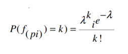
Photon Noise is also called as Poisson Noise. Due to the statistical nature of electromagnetic waves the appearance of this noise is seen. The rays emitted from x-ray and gamma rays are injected in patient’s body from its source. Result gathered image has spatial and temporal randomness. This noise is also called as quantum noise or shot noise. This noise obeys the Poisson distribution and is given as
Poisson-Gaussian Noise
They are arosed in Magnetic Resonance Imaging (MRI).It is a combination of two models which specifies the quality of MRI recipient signal in terms of visual appearances and strength.The Poisson Gaussian noise model is given as:
Z(j,k)=α* P˅α(j,k) + N˅α(j,k)
P˅α=Poisson-distribution
N˅α=Gaussian distribution
µ˅α1=mean
µ˅α2=zero mean
Poisson-distribution is estimated using mean at given level α>0 µ and Gaussian-distribution counted at level α > 0 using zero mean and variance. Poisson image is quantitatively added to underlying original image to evaluate mean.

Figure 4: Poisson-Gaussian Noise
Structured Noise
They are periodic and a-periodic in nature. They may or may not be stationary (fixed amplitude, frequency and phase). There are two types of Noise presents in communication channel unstructured noise(u) and structured noise(s) also called as low rank noise.
Structured noise model is given as:
y(n) = x(n,m) + v(n)
Y(n) = H(n,m) * θ(m) + S(n,t)*φ(t) + v(n)
n = rows,
m = columns,
y = received image,
H = Transfer function of linear system,
S = Subspace,
t = rank in subspace,
φ= underlying process ,
θ= signal parameter

Figure 5: Structured Noise
Gamma Noise
They are seen in the laser based images. The Gamma Noise follows the Gamma distribution. The Gamma Noise model is given as:
		P(g)= { a^(b) g^(b-1) e^(-ag) /( b-1)! for g>=0
				0 for g<0}
Mean=b/a
Variance=b/a^2

Figure 6: Gamma Distribution
Rayleigh Noise
They are presents in radar range images.It follows the probability density function and the model is given as
		P(g)={2/b(g-a)e^((-(g-a)^2)/b) for g>=a
			 0 for g<a}
Mean = a + square_root (πb/4)
Variance = b(4-π)/4

Figure 7: Rayleigh Noise

Figure 8: Rayleigh Distribution
Noise is seen during image acquisition and transmission which is characterized by the various noise model. So it is much important to learn about the Noise Model because without them we cannot elaborate and perform the denoising actions. Noise models are basically designed on probability density function which uses mean and variance.
Comments