Author – Saumya Arora
Model-free reinforcement learning has been successfully applied to a range of challenging problems and has recently been extended to handle large neural network policies and value functions. However, the sample complexity of model-free algorithms, particularly when using high-dimensional function approximators, tends to limit their applicability to physical systems. In this paper, we explore algorithms and representations to reduce the sample complexity of deep reinforcement learning for continuous control tasks.In this work, we make the first attempt to understand Deep-Q-Learning from both algorithmic and statistical perspectives. In specific, the work is mainly focused on Deep-Q-Network Algorithm and its main parts i.e., Initializing the main target and neural network, choose an action using Epsilon Greedy and Update your network weights using Bellman Equation.
TABLE OF CONTENTS: -
REINFORCEMENT LEARNING.
Q LEARNING.
DEEP-Q-LEARNING.
DEEP-Q-NETWORK ALGORITHM:
Initialize your main and target neural networks.
Choose an action using the Epsilon-Greedy Strategy.
Update your network weights using the Bellman Equation.
EXPERIENCE REPLAY.
BELLMAN EQUATION:
Value iteration.
Policy iteration.

Figure-1
WHAT IS REINFORCEMENT LEARNING?
We must understand Reinforcement Learning before starting Deep Q Learning.
Reinforcement Learning is an area of machine learning which is concerned with low intelligent agents who ought to take actions in an environment to maximize the notion of cumulative reward. It is one of the three basic paradigms, alongside supervised learning and unsupervised learning.
Reinforcement Learning differs from supervised learning in not needing labeled input/output pairs to be presented and in not needing sub optional actions to be explicitly corrected. Instead, it focuses on finding a balance between exploration (of uncharted territory) and exploitation (of current knowledge).
WHAT IS Q LEARNING?
It is a basic form of Reinforcement Learning which uses Q -values (also called action values) to iteratively improve the behavior of the learning agent. It's considered off policy because the Q learning function learns from actions that are outside the current policy, like taking random actions, and therefore a policy isn't needed. ‘Q’ in Q-Learning stands for quality. Quality in this case represents how useful a given action is in gaining a future reward.
WHAT IS DEEP-Q-LEARNING?
Deep-Q-Learning uses user experience relay to learn in small batches to avoid skewing the dataset distribution of different states, actions, rewards, and next states that the neural network will see. Importantly the agent doesn't need to train after each step. The process of Deep-Q-learning crates an exact matrix for the working agent which can be used to maximize its reward in the long run. Although this approach is not wrong in itself, this is only practical for very small environments and quickly losses its feasibility when the number of states and actions in the environment increases.
The solution for the above problem comes from the realization that the values in the matrix only have relative importance i.e., the values only have importance concerning other values. Thus, this thinking leads us to Deep-Q-Learning which uses a deep neural network to approximate the values. This approximation of values doesn’t hurt as long as the relative importance is preserved. The basic working step for Deep-Q-Learning is that the initial state is fed into the neural network and it returns the Q-values of all possible actions as on output.
THE DEEP-Q-NETWORK ALGORITHM: -
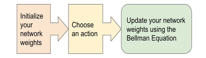
Figure-2
The algorithm mainly consists of 3 parts: -
Initialize your main and target neural networks.
Choose an action using the Epsilon-Greedy Strategy.
Update your network weights using the Bellman Equation.
Explanation:
1.Initialize your target and main neural networks: -
Deep learning replaces the regular Q-Table with a neural network, rather than mapping a state-action pair to a Q-value, a neural network maps inputs states to (action, Q-value) pairs.
1.The importance of effective initialization: -
To build a machine learning algorithm, usually, you had to define an architecture (e.g., logistic regression, support vector machine, neural network, etc.) and train it to learn parameters. Here is a common training process for a neural network: -
Initialize the parameters.
Choose an optimizing algorithm.
Repeat these steps:
Forward propagate an input.
Compute the cost function.
Compute the gradients of the cost concerning parameters using backpropagation.
Update each parameter using gradients, according to the optimization algorithm.
Then given a new data point you can use the model to predict its class. The initializing step can be critical to the model’s ultimate performance and it requires the right method.
2.The problem of exploding or vanishing gradients: -
Consider this 9-layer neural network :

Figure-3
At every iteration of the optimization loop (forward, cost, backward, update), we observe that backpropagated gradients are either amplified or minimized as you move from the output layer towards the input layer. This result makes sense if you consider the following example. Assume all the activation functions are linear (identity function). Then the output activation is:

Were,
L=10

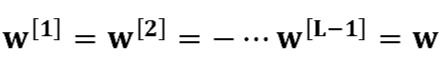
are all matrices of size (2,2) because layers [1] to [L-1] have 2 neurons and receive 2 inputs. With this in mind, and for illustrative purposes, if we assume
then, the output prediction is

Case 1: A too-large initialization leads to exploding gradients.
Consider the case where every weight is initialized slightly larger than the identity matrix.
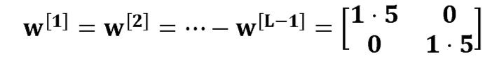
This simplifies to

And the values of an [l] increase exponentially with l. When these activations are used in backward propagation, this leads to the exploding gradient problem. That is, the gradients of the cost with the respect to the parameters are too big. This leads the cost to oscillate around its minimum value.
Case 2: A too-small initialization leads to vanishing gradients.
Similarly, consider the case where every weight is initialized slightly smaller than the identity matrix.

This simplifies to

And the values of the activation a[l] decrease exponentially with l. When these activations are used in backward propagation, this leads to the vanishing gradient problem. The gradients of the cost concerning the parameters are too small, leading to convergence of the cost before it has reached the minimum value.
All in all, initializing weights with inappropriate values will lead to divergence or a slow-down in the training of your neural network. Although we illustrated the exploding/vanishing gradient problem with simple symmetrical weight matrices, the observation generalizes to any initialization values that are too small or too large.
3.How to find appropriate initialization values:
To prevent the gradients of the network’s activations from vanishing or exploding, we will stick to the following rules of thumb:
The mean of the activations should be zero.
The variance of the activations should stay the same across every layer.
Under these two assumptions, the backpropagated gradient signal should not be multiplied by values too small or too large in any layer. It should travel to the input layer without exploding or vanishing. More concretely, consider a layer ll. Its forward propagation is:

We would like the following to hold:

Ensuring zero-mean and maintaining the value of the variance of the input of every layer guarantees no exploding/vanishing signal, as we'll explain in a moment. This method applies both to forward propagation (for activations) and backward propagation (for gradients of the cost to activations). The recommended initialization is Xavier initialization (or one of its derived methods), for every layer L.

In other words, all the weights of layer l are picked randomly from a normal distribution with mean μ=0 and variance

where,

is the number of neurons in layer l-1. Biases are initialized
with zeros.
4.Justification for Xavier initialization:
Xavier Initialization keeps the variance the same across every layer. Here we will assume that our layer’s activations are normally distributed around zero. Sometimes it helps to understand the mathematical justification to grasp the concept, but you can understand the fundamental idea without the math. A common math trick is to extract the summation outside the variance. To do this, we must make the following three assumptions:
Weights are independent and identically distributed.
Inputs are independent and identically distributed..
Weights and inputs are mutually independent.
5. Mapping of States (ACTION, Q-VALUES) Pairs:

Figure-4
The main and target neural networks map input states to an (action, q-value) pair. In this case, each output node (representing an action) contains the action’s q-value as a floating-point number.
2.Choose an action using the Epsilon-Greedy Exploration Strategy: -

Figure-5
In epsilon-greedy action selection, the agent uses both exploitations to take advantage of prior knowledge and exploration to look for new options. The epsilon greedy approach selects the action with the highest estimated reward most of the time. The aim is to have a balance to have some room for trying new things, sometimes contradicting what we have already learned.
With a small probability of what we choose to explore, i.e., not to exploit what we have learned so far. In this case, the action is selected randomly, independent of the action-value estimates. If we make infinite trials, each action is taken an infinite number of times. Hence, the epsilon-greedy action selection policy discovers the optimal actions for sure.
An epsilon-greedy algorithm is easy to understand and implement. Yet it’s hard to beat and works as well as more sophisticated algorithms. We need to keep in mind that using other action selection methods is possible. Depending on the problem at hand, different policies can perform better.
For example, the SoftMax action selection strategy controls the relative levels of exploration and exploitation by mapping values into action probabilities. Here we use the same formula from the SoftMax activation function, which we use in the final layer of classifier neural networks.
1). Epsilon-Greedy Q-learning Parameters: -
In this type of method, we have three parameters i.e., alpha gamma, and the third one is epsilon (epsilon greedy action selection).
ALPHA (α): - Similar to other machine learning algorithms, alpha (α) defines the learning rate or step size. As we can see from the equation above, the new Q-value for the state is calculated by incrementing the old Q-value by alpha multiplied by the selected action’s Q-value. Alpha is a real number between zero and one (0 < α ≤ 1). If we set alpha to zero, the agent learns nothing from new actions. Conversely, if we set alpha to 1, the agent completely ignores prior knowledge and only values the most recent information. Higher alpha values make Q-values change fast.
GAMMA (ɣ): - Gamma (ɣ) is the discount factor. In Q-learning, gamma is multiplied by the estimation of the optimal future value. The next reward’s importance is defined by the gamma parameter. Gamma is a real number between 0 and 1 (0 ≤ ɣ ≤ 1). If we set gamma to zero, the agent completely ignores the future rewards. Such agents only consider current rewards. On the other hand, if we set gamma to 1, the algorithm would look for high rewards in the long term. A high gamma value might prevent conversion: summing up non-discounted rewards leads to having high Q-values.
EPSILON (): -Epsilon () parameter is related to the epsilon-greedy action selection procedure in the Q-learning algorithm. In the action selection step, we select the specific action based on the Q-values we already have. The epsilon parameter introduces randomness into the algorithm, forcing us to try different actions. This helps not getting stuck in a local optimum. If epsilon is set to 0, we never explore but always exploit the knowledge we already have. On the contrary, having the epsilon set to 1 forces the algorithm to always take random actions and never use past knowledge. Usually, epsilon is selected as a small number close to 0.
3.Update your Network Weights using the Epsilon Equation: -
After choosing an action, it’s time for the agent to perform the action and update the Main and Target networks according to the Bellman equation. Deep Q-Learning agents use Experience Replay to learn about their environment and update the Main and Target networks. To summarize, the main network samples and trains on a batch of past experiences every 4 steps. The main network weights are then copied to the target network weights every 100 steps.
Experience Replay: -
Experience Replay is the act of storing and replaying game states (the state, action, reward, next state) that the RL algorithm can learn from. Experience Replay can be used in Off-Policy algorithms to learn in an offline fashion. Off-policy methods can update the algorithm's parameters using saved and stored information from previously taken actions. Deep Q-Learning uses Experience Replay to learn in small batches to avoid skewing the dataset distribution of different states, actions, rewards, and next states that the neural network will see. Importantly, the agent doesn't need to train after each step. In our implementation, we use Experience Replay to train on small batches once every 4 steps rather than every single step. We found this trick to help speed up our Deep Q-Learning implementation.
BELLMAN EQUATION: -

Figure-6
A Bellman equation is a necessary condition for optimality associated with the mathematical optimization method known as dynamic programming. It writes the "value" of a decision problem at a certain point in time in terms of the payoff from some initial choices and the "value" of the remaining decision problem that results from those initial choices. This breaks a dynamic optimization problem into a sequence of simpler subproblems, as Bellman's “principle of optimality” prescribes.
The term 'Bellman equation' usually refers to the dynamic programming equation associated with discrete-time optimization problems. In continuous-time optimization problems, the analogous equation is a partial differential equation that is called the Hamilton–Jacobi–Bellman equation.
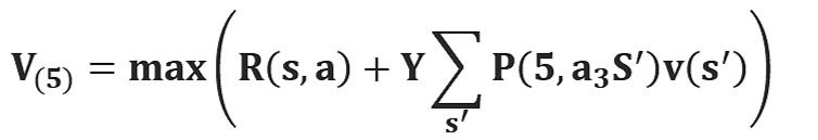
In discrete-time, any multi-stage optimization problem can be solved by analyzing the appropriate Bellman equation. The appropriate Bellman equation can be found by introducing new state variables (state augmentation). However, the resulting augmented-state multi-stage optimization problem has a higher dimensional state space than the original multi-stage optimization problem - an issue that can potentially render the augmented problem intractable due to the “curse of dimensionality”. Alternatively, it has been shown that if the cost function of the multi-stage optimization problem satisfies a "backward separable" structure then the appropriate Bellman equation can be found without state augmentation. The optimal value function V*(S) yields the maximum value.
The value of a given state is

equal to the max action (action which maximizes the value) of the reward of the optimal action in the given state and add a discount factor multiplied by the next state’s Value from the Bellman Equation.
Let's understand this equation, V(s) is the value for being in a certain state. V(s’) is the value for being in the next state that we will end up in after taking action a. R (s, a) is the reward we get after taking action an in states. As we can take different actions so we use maximum because our agent wants to be in the optimal state. γ is the discount factor as discussed earlier. This is the Bellman equation in the deterministic environment. It will be slightly different for a non-deterministic environment or a stochastic environment.
In a stochastic environment when we take an action it is not confirmed that we will end up in a particular next state and there is a probability of ending in a particular state. P (s, a, s’) is the probability of ending is state’s from s by taking action a. This is summed up to a total number of future states. For example, if by taking an action we can end up in 3 states s₁, s₂, and s₃ from states with a probability of 0.2, 0.2, and 0.6. The Bellman equation will be
V(s) = maxₐ (R (s, a) + γ(0.2*V(s₁) + 0.2*V(s₂) + 0.6*V(s₃) )
We can solve the Bellman equation using a special technique called dynamic programming.
Dynamic Programming:
Dynamic programming (DP) is a technique for solving complex problems. In DP, instead of solving complex problems one at a time, we break the problem into simple subproblems, then for each sub-problem, we compute and store the solution. If the same subproblem occurs, we will not recompute, instead, we use the already computed solution. We solve a Bellman equation using two powerful algorithms:
Value Iteration.
Policy Iteration.
Value Iteration: -

Figure-7
In value iteration, we start with a random value function. As the value table is not optimized if randomly initialized, we optimize it iteratively.
Calculating the V-value with loops: -Let’s see how these cases are solved with a simple Environment with two states, state 1 and state 2, that presents the following environment’s states transition diagram:

Figure-8
We only have two possible transitions: from state 1 we can take only an action that leads us to state 2 with Reward +1 and from state 2 we can take only an action that returns us to state 1 with a Reward +2. So, our Agent’s life moves in an infinite sequence of states due to the infinite loop between the two states.
Suppose that we have a discount factor γ<1, let’s say 0,9, and remember from the previous post that the optimal value of the state is equal to that of the action that gives us the maximum possible expected immediate reward, plus the discounted long-term reward for the next state:

In our example, since there is only one action available in each state, our Agent has no other option and therefore we can simplify the previous formula as:

For instance, if we start from state 1, the sequence of states will be [1,2,1,2,1,2, …], and since every transition from state 1 to state 2 gives us a Reward of +1 and every back transition gives us a Reward of +2 the sequence of Rewards will be [+1, +2, +1, +2, +1, +2, …]. Therefore, the previous formula for state 1 becomes:

Strictly speaking, it is impossible to calculate the exact value of our state, but with a discount factor γ= 0,9, the contribution of a new action decreases over time. For example, for sweep i=37 the result of the formula is 14.7307838, for sweep i=50 the result is 14.7365250 and for sweep i=100 the result is 14.7368420. That means that we can stop the calculation at some point (e.g. at i=50) and still get a good estimate of the V-value, in this case, V(1) = 14.736.
The Value Iteration Algorithm:-The preceding example can be used to get the gist of a more general procedure called the Value Iteration algorithm (VI). This allows us to numerically calculate the values of the states of Markov decision processes, with known transition probabilities and rewards. The idea behind the Value Iteration algorithm is to merge a truncated policy evaluation step (as shown in the previous example) and a policy improvement into the same algorithm.
The Value Iteration algorithm computes the optimal state value function by iteratively improving the estimate of V(s). The algorithm initializes V(s) to arbitrary random values. It repeatedly updates the Q (s, a) and V(s) values until they converge. Value Iteration is guaranteed to converge to the optimal values. The following pseudo-code express this proposed algorithm:

Figure-9
Estimation of Transitions and Rewards:-In practice, this Value Iteration method has several limitations. First of all, the state space should be discrete and small enough to perform multiple iterations over all states. This is not an issue for our Frozen-Lake Environment but in a general Reinforcement Learning problem, this is not the case. Another essential practical problem arises from the fact that to update the Bellman equation, the algorithm requires knowing the probability of the transitions and the Reward for every transition of the Environment.
Estimation of Rewards:-Estimate Rewards is the easiest part since Rewards could be used as they are. We just need to remember what reward we got on the transition from s to s’ using action a.
Estimation of Transitions:-To estimate transitions is also easy, for instance by maintaining counters for every tuple in the Agent’s experience (s, a, s’) and normalize them. For instance, we can create a simple table that keeps the counters of the experienced transitions. The key of the table can be a composite “state” + “action”, (s, a), and the values of each entry there is the information about target states, s’, and a count of times that we have seen each target state, c.
Let’s look at an example. Imagine that during Agent’s experience, in a given state s0 it has executed an action several times and it ends up c1 times in state s1 and c2 times in state s2. How many times we have switched to each of these states is stored in our transition table. That is, the entry (s,a) in the table contents {s1: c1, s2: c2}. Perhaps visually you can more easily see the information contained in the table for this example:
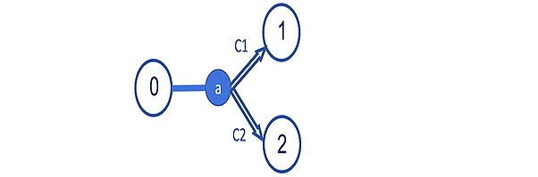
Figure-10
Then, it is easy to use this table to estimate the probabilities of our transitions. The probability that the action will take us from state 0 to state 1 is c1 / (c1 + c2) and that the action will take us from state 0 to state 2 c2 / (c1 + c2).
For example, imagine that from a state 0 we execute action 1 ten times, and after 4 times it will lead us to state 1, and after 6 times it will lead us to state 2. For this particular example, the entry with the key (0, 1) in this table contents {1: 4, 2: 6}. And this represents that the probability of transition from state 0 to state 1 is 4/10, that is, 0.4, and that of state 0 to state 2 of 6/10, that is, 0.6. With this information estimated from the experience of the Agent, we already have all the necessary information to be able to apply the Value Iteration algorithm.
Policy Iteration:-

In Policy Iteration the actions which the agent needs to take are decided or initialized first and the value table is created according to the policy. In policy iteration algorithms, we start with a random policy, then find the value function of that policy (policy evaluation step), after then we find a new (improved) policy based on the previous value function, and so on. In this process, each policy is guaranteed to be a strict improvement over the previous one (unless it is already optimal). Given a policy, its value function can be obtained using the Bellman operator. Let us assume we have a policy (𝝅: S → A) that assigns an action to each state. Action 𝝅(s) will be chosen each time the system is at state s.
Evaluate a given policy (e.g., initialize policy arbitrarily for all states s ∊ S) by calculating the value function for all states s ∊ S under the given policy:

Value function = the expected reward collected at the first step + expected discounted value at the next state
Improve policy to find better action for state s ∊ S.

Repeat step 1,2 until value function converge to optimal value function.
Conclusion: -
From both the methods analytical and statistical we found that Deep-Q-Learning is way better than Reinforcement Learning and after adding Deep Learning in Reinforcement Learning we have come across most of the bottlenecks/ disadvantages of Reinforcement Learning which have successfully been solved by Deep-Q-Learning or Deep Reinforcement Learning. No doubt even there are some things which can’t be even solved by Deep-Q-Learning but till now it has an upper hand on Reinforcement Learning.
Codes: -
Initialize your main and target neural networks, Epsilon-Greedy Strategy, Bellman Equation (Jupyter notebook).
Resources: -
Initialization the main Neural Network :https://www.deeplearning.ai/ai-notes/initialization/
Main part :https://www.analyticsvidhya.com/blog/2019/04/introduction-deep-q-learning-python/
Forarticles:https://scholar.google.co.in/scholarq=deep+q+learning&hl=en&as_sdt=0&as_vis=1&oi=scholart
Main part :http://proceedings.mlr.press/v48/gu16.pdf
Reinforcement learning: https://www.geeksforgeeks.org/what-is-reinforcement-learning/
Q learning:https://www.geeksforgeeks.org/q-learning-in-python/#:~:text=Q%2DLearning%20is%20a%20basic,the%20action%20at%20the%20state%20.
Epsilon Greedy: https://www.baeldung.com/cs/epsilon-greedy-q-learning#:~:text=In%20epsilon%2Dgreedy%20action%20selection,balance%20between%20exploration%20and%20exploitation.
Bellman Equation:https://medium.com/analytics-vidhya/bellman-equation-and-dynamic-programming-773ce67fc6a7
Github:https://github.com/saumyaarora80/deep-q-learning-saumya-arora-
Commenti