EXPECTATION MAXIMATION ALGORITHM

Sep 19, 20216 min read

Author : Chetan Omprakash Khandelwal

The problem with parameter estimation based algorithm is that it becomes more complicated because direct access to the data that is necessary to estimate the parameters in not possible Or in some cases some data points are missing. This type of problem arises when outcomes are group together for the example in binning or histogram operation. There can be data dropout or clustering in such a way that number of underlying data points are unknown. Then for such type of problem EM (Expectation Maximization) algorithm is best approach that it produces maximum-likelihood (ML) estimates of parameters when there is a many-to-one mapping from an underlying distribution to the distribution governing the observation. The EM algorithm consists of two major steps: an expectation step, followed by a maximization step. That we will discuss below.

Contents :–

Existing techniques for clustering.
Limitation of K-means Algorithm.
Introduction to Gaussian mixture model.
Maximum likelihood Estimation for Gaussian mixture model and it’s Limitation.
Expectation Maximization Algorithm.
Detailed Explanation of the Algorithm.

Existing Techniques for Clustering:-

There are Different methods available for Clustering like-

1) K -Means Clustering-

Figure-1

2) Gaussian Mixture Models-

Figure-2

Limitation of K-Means Algorithm:-

One of the major drawback coming from k-means algorithm is that is does the hard assignment and not soft assignment means each point in k-means contributes to particular centroid. In short we can say that fractional clustering in k-means algorithm is not possible. If in case we don’t know the source of the data points we can’t use k-means algorithm over there. So we need some algorithm that can give it’s little mass to every centroid but it give more mass to centroid it is more associated with.

Introduction to Gaussian mixture model:-

Mixture model is a probabilistic model for representing the presence of subpopulations within an overall population. It represents the probability distribution of observation in overall population. GMM or Gaussian mixture model is a mixture model that uses combination probability distribution and also requires the estimation of mean and standard deviation parameters. In simple words the clusters in GMM comes from different Gaussian distribution or we can say mixture of several Gaussian distribution. It is joined probability distribution. The most commonly used technique for Gaussian mixture model is maximum likelihood algorithm.

Figure-3

Maximum Likelihood Estimation:-

This is the most common technique used for Gaussian mixture model. Maximum likelihood estimation is a method that determines values for the parameters of a model. The parameter values are found such that they maximize the likelihood that the process described by the model produced the data that were actually observed.

For Better understanding let’s take a example-

Suppose we have 10 data points for certain process and those 10 points are given as shown below.

Figure-4

The first important part is we first have to decide which model we think best describes the process of generating the data. We should have good idea which model to use. For these data we’ll assume that the data generation process can be adequately described by a Gaussian (normal) distribution. We have made this decision by visual inspection by looking at points as most of them are clustered around the Centre.

The mean, μ, and the standard deviation, σ. Different values of these parameters result in different curves (just like with the straight lines above). We want to know which curve was most likely responsible for creating the data points that we want (See figure below). Maximum likelihood estimation is a method that will find the values of μ and σ that result in the curve that best fits the data.

Figure-5

Limitations of Maximum likelihood Estimation:-

Maximum likelihood estimation can find the “best fit” model for a set of data, it doesn’t work particularly well for incomplete data sets.
MLE accumulates all of the data first and then uses that data to construct the most likely model. Unlike Expectation Maximization Algorithm that takes a guess at the parameters first—accounting for the missing data.

Expectation maximization Algorithm :-

The Expectation-Maximization (EM) algorithm is an iterative way to find maximum-likelihood estimates for model parameters when the data is incomplete or has some missing data points or has some hidden variable. The EM algorithm can be used to estimate latent variables, like ones that come from mixture distributions (you know they came from a mixture, but not which specific distribution). An initial guess is made for the model’s parameters and a probability distribution is created. This algorithm chooses some random values for missing data and estimates new data set. This algorithm solves the problem of latent (Hidden variable) in Gaussian mixture model and find the way to complete the missing data set.

This is sometimes called the “E-Step” for the “Expected” distribution.

Flowchart:-

Figure-6

Algorithm:-

Given a set of incomplete data, start with the set of initialized parameters.
Expectation step or E-Step- In this method by using the dataset which we have we try to estimate or guess the values of missing data. After this step we have complete data with no missing values.
Maximization step or M-step- In this step the new data generated from the expectation step is used to update the parameters.
Repeat step 2 and 3 until the convergence.

The EM Algorithm always improves a parameter’s estimation through this multi-step process. However, it sometimes needs a few random starts to find the best model because the algorithm can hone in on a local maxima that isn’t that close to the (optimal) global maxima.

Detailed Explanation of the Algorithm:-

For better understanding we will see Ector’s problem:

Suppose that in an image pattern-recognition problem, there are two general classes to be distinguished: a class of dark objects and a class of light objects. The class of dark object is further divided into two type of shapes round and square. Using a pattern recognizer, it is desired to determine the probability of a dark object. Let the random variable X1 represent the number of round dark objects, X2 represent the number of square dark objects, and X3 represent the number of light objects, and let [x1, x2, x3]’ = x be the vector of values the random variables take for some image.

Probability of the classes may be written as:

W here p is an unknown parameter of the distribution and n = x1+x2+x3. The notation f(x1,x2,x3|p) is typical throughout the article; it is used to indicate the probability function which may be either a probability density function (pdf) or a probability mass function (pmf). A feature extractor is employed that can distinguish which objects are light and which are dark, but cannot distinguish shape . Let [y1,y2]T be the number of dark and light object detected. y, so that y1 = x1 + x2 and y2 = x3, and the corresponding variable be Y1 and Y2. There is a many-to-one mapping between (x1,x2} and y1. The EM algorithm is specifically designed for problems with such many-to-one mapping.

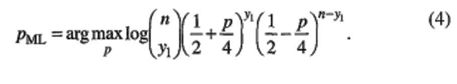
(g is used to indicate the probability function for the observed data.) From the observation of y1 and y2, compute the ML estimate of p,

Where ‘argmax’ means the value that maximizes the function.

Now while starting EM algorithm we will not directly go to ML estimate. Taking the logarithm of the likelihood often simplifies the maximization and yields equivalent results since log is an increasing function

The basic idea behind the EM is that even though we do not know x1 and x2, knowledge of the underlying distribution f(x1, x2, x3|p) can be used to determine an estimate for p. This is done by first estimating the underlying data, then using these data to update our estimate of the parameter. This is repeated until convergence. e. Let p[k] indicate the estimate of p after the kth iteration, k = 1,2, .... An initial parameter value p[0] is assumed. The algorithm consists of two major steps.

1) Expectation Step [E-Step]:

Compute the expected value of the x data using the current estimate of the parameter and the observed data. The expected value of x1, given the measurement y1 based upon the current estimate of the parameter, may be computed as:

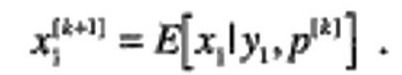
Figure-7

In the current example, x3 is known and does not need to be computed.

2) Maximization Step [M-Step]:

In this we are going to use the data form expectation step and as if it were actually measured data to determine an ML estimate of the parameter. This data is sometimes called as “imputed” data. In the following example the x1[k+1] and x2[k+2] are imputed and x3 is available. The machine learning parameters are obtained by taking the derivative of log f(x1[k+1], x2[k+2], x3 |p) with respect to p, equating it to zero, and solving for p.

The EM algorithm consists of iterating Equation (6) and (7) until convergence. Intermediate computation and storage may be eliminated by substituting Eq. (6) into Eq. (7) to obtain a one-step update.

Output-

Before EM algorithm-

Figure-8

After using the EM algorithm-

Figure-9

GitHub URL:-

https://github.com/Chetank2830/Machine-learning.git

Madras Scientific Research Foundation