Gaussian processes are used as standards for reasoning about functions having partial knowledge. It is generally used in decision-making scenarios to represent predictive uncertainties. In decision-making, well-calibrated predictive uncertainty plays an important role in balancing. Bayesian methods naturally strike this balance. Naïve approaches are statistically better but require hectic solutions of linear systems at run times. The approximation strategies based on Fourier features are faster and do not use costly matrices but misrepresent predictive posteriors.
There are two types of Gaussian Processes:
Function - space approximations to GPs - Here the predictions of Gaussian Processes are done based on distributions of functions.
Weight - space approximations to GPs - Here reason of functions is done based on the weighted sum of basis functions.
Gaussian (GP) procedures are a standardized learning approach designed to skip backward and potential planning problems.

Advantages of Gaussian procedures :
Prediction includes visibility (at least standard characters).
This prediction is possible (in Gaussian) so that one can calculate strong confidence intervals and decide based on what one can reject (online estimates, flexibility) of the forecast in a particular region of interest.
Disadvantages of Gaussian procedures :
They do not exceed, that is, they use all samples/data to make predictions.
They lose efficiency in high-density spaces - i.e. when the number of features exceeds a few tens.
An effective sample from a recent Gaussian process is suitable for practical application. Under Matheron's rule, we unravel the following, which allows us to simulate activities from the Gaussian process after a limited period.
Gaussian systems (GPs) play a very important role in many machine learning algorithms. For example, successive decision-making strategies such as the use of Bayesian use GPs to represent the results of various actions. Actions are then selected by increasing the conditional expectation of the performance of the selected reward concerning the GP posterior. These expectations are often unattainable when it comes to clear wage jobs, but they are probably well-balanced by Monte Carlo methods.
Gaussian Regression (GPR) Process
The Gressus Process Regressor uses Gaussian (GP) procedures for regression purposes. For this, pre-GP needs to be clarified. The previous definition is considered to be static and zero (for normalize_y = False) or the definition of training data (for normalize_y = True). The previous covariance is defined by transferring a kernel object. Kernel hyperparameters are adjusted during the installation of the Gaussian Process Regressor by increasing the entry-level (log-marginal-likelihood (LML) based on the transmitted optimizer. by specifying a n_restarts_optimizer. The first run is always run from the original kernel hyperparameter values;
The level of sound in the target can be determined by transmitting it with a parameter alpha, either worldwide as a scale or with a data point.
Importance of the Gaussian Process Transfer:
Allows predictions without pre-measurement (depending on GP prior).
Provides an additional sample_y (X), which examines samples taken from GPR (before or after) input provided.
Learn the importance of features.
Make offline predictions.
Guess the Gaussian distribution over its output.
Gaussian Process Separation (GPC)
The Gaussian Processes Classifier is a machine learning algorithm. Gaussian systems are designed for the distribution of Gaussian distribution opportunities and can be used as a basis for complex non-parametric applications for classification and regression.
Kernels for Gaussian processes:
Standard Kernels
Basic Kernels
Types of Standard Kernels
Squared Exponential Kernel
Rational Quadratic Kernel
Periodic Kernel
Linear Kernel
Squared Exponential Kernel:
It is of the form
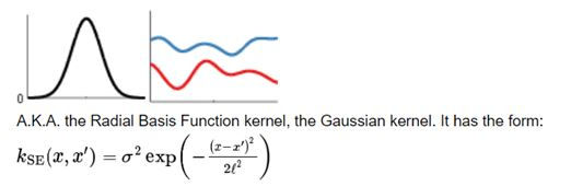
It also has only two parameters:
The length scale ℓ determines the length of the 'wiggles' in your function. In general, you won't be able to extrapolate more than ℓ units away from your data.
The output variance σ2 determines the average distance of your function away from its mean. Every kernel has this parameter out in front; it's just a scale factor.
Rational Quadratic Kernel:
It is of the form

The parameter α determines the relative weighting of large-scale and small-scale variations. When α→∞, the RQ is identical to the SE.
Periodic Kernel:
It is of the form:

The period p simply determines the distance between repetitions of the function.
The lengthscale ℓ determines the lengthscale function in the same way as in the SE kernel.
Linear Kernel:
It is of the form:

The parameters of the linear kernel are about specifying the origin:
The offset c determines the x-coordinate of the point that all the lines in the posterior go though. At this point, the function will have zero variance (unless you add noise)
The constant variance σb2 determines how far from 0 the height of the function will be at zero
.
Basic Kernels:
Constant Kernel :
It is used as part of a Product kernel where it scales the magnitude of the other factor (kernel) or as part of a Sum kernel, where it modifies the mean of the Gaussian process. It depends on a parameter constant_value.

Multiplying kernels :
Multiplying together kernels is the standard way to combine two kernels, especially if they are defined on different inputs to your function. Roughly speaking, multiplying two kernels can be thought of as an AND operation.
Linear times periodic :
A linear kernel times a periodic result in functions which are periodic with increasing amplitude as we move away from the origin.

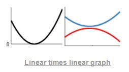
Linear times linear:
A linear kernel times another linear kernel results in functions which are quadratic.
Multi-dimensional product:

Multiplying two kernels which each depend only on a single input dimension results in a prior over functions that vary across both dimensions. That is, the function value f(x,y). f(x,y) is only expected to be similar to some other function value f(x′,y′) if x is close to x′ AND y is close to y′.
These kernels have the form : Kproduct (x, y, x′, y′) = kx ( x, x′ ) ky ( y, y′)
White Kernel :
It is as part of a sum-kernel where it explains the noise-component of the signal. It’s main parameter is noise_level.

Adding two Kernels:
Adding two kernels can be thought of as an OR operation.
Linear plus periodic:
A linear kernel plus a periodic result in functions which are periodic with increasing mean as we move away from the origin.

Adding across dimensions:

Adding kernels which each depend only on a single input dimension results in a prior over functions which are a sum of one-dimensional functions, one for each dimension. That is, the function f(x,y). f(x,y) is simply a sum of two functions fx(x)+fy(y).
These kernels have the form : k additive(x, y, x′, y′) = kx(x, x′ ) + ky(y, y′ )
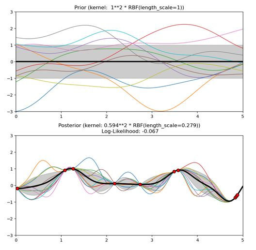
Radial basis function (RBF) Kernel:
It is also known as squared exponential kernel(explained earlier). It is given by:

where d(.,.) is the Euclidean distance.
Rational Quadratic Kernel :
It is a type of RBF with difference in the length-scale.


Exponential-Sine Squared Kernel:
The ExpSineSquared kernel allows modeling periodic functions. It is parameterized by a length-scale parameter l>0 and a periodicity parameter p>0. Only the isotropic variant where l is a scalar is supported at the moment. The kernel is given by:


Dot Product Kernel
The DotProduct kernel is non-stationary and can be obtained from linear regression.
The DotProduct kernel is invariant to a rotation of the coordinates about the origin, but not translations. It is given by:


References:
Comments