RIDGE REGRESSION

Sep 19, 20216 min read

Author -Abhishek A L.

A Ridge regressor is basically a regularized version of Linear Regressor. i.e. to the original cost function of linear regressor we add a regularized term which forces the learning algorithm to fit the data and helps to keep the weights lower as possible. This blog tries to explain related to topic out there, while majorly following on explaining ridge regression with example codes.

What is ridge regression?

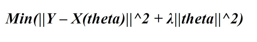
Ridge regression is a model tuning method that is used to analyze any data that suffers from multicollinearity. This method performs L2 regularization. When the issue of multicollinearity occurs, least-squares are unbiased, and variances are large, this results in predicted values to be far away from the actual values. The cost function for ridge regression:

Lambda is the penalty term. λ given here is denoted by an alpha parameter in the ridge function. So, by changing the values of alpha, we are controlling the penalty term. Higher the values of alpha, bigger is the penalty and therefore the magnitude of coefficients is reduced.

It shrinks the parameters. Therefore, it is used to prevent multicollinearity.
It reduces the model complexity by coefficient shrinkage.

Why Use Ridge Regression?

The advantage of ridge regression compared to least squares regression lies in the bias-variance trade-off. Recall that mean squared error (MSE) is a metric we can use to measure the accuracy of a given model and it is calculated as:

The basic idea of ridge regression is to introduce a little bias so that the variance can be substantially reduced, which leads to a lower overall MSE. to illustrate this, consider the following chart:

Figure-1

Notice that as λ increases, variance drops substantially with very little increase in bias. Beyond a certain point, though, variance decreases less rapidly and the shrinkage in the coefficients causes them to be significantly underestimated which results in a large increase in bias.

We can see from the chart that the test MSE is lowest when we choose a value for λ that produces an optimal trade-off between bias and variance. When λ = 0, the penalty term in ridge regression has no effect and thus it produces the same coefficient estimates as least squares. However, by increasing λ to a certain point we can reduce the overall test MSE.

Figure-2

This means the model fit by ridge regression will produce smaller test errors than the model fit by least squares regression. Ridge Regression Models For any type of regression machine learning models, the usual regression equation forms the base which is written as:

Y = XB + e

Where Y is the dependent variable, X represents the independent variables, B is the regression coefficients to be estimated, and e represents the errors are residuals. Once we add the lambda function to this equation, the variance that is not evaluated by the general model is considered. After the data is ready and identified to be part of L2 regularization, there are steps that one can undertake.

Standardization:

In ridge regression, the first step is to standardize the variables (both dependent and independent) by subtracting their means and dividing by their standard deviations. This causes a challenge in notation since we must somehow indicate whether the variables in a particular formula are standardized or not. As far as standardization is concerned, all

ridge regression calculations are based on standardized variables. When the final regression coefficients are displayed, they are adjusted back into their original scale. However, the ridge trace is on a standardized scale.

Bias and variance trade-off:

Bias and variance trade-off is generally complicated when it comes to building ridge regression models on an actual dataset. However, following the general trend which one needs to remember is:

The bias increases as λ increases.
The variance decreases as λ increases.

Assumptions of Ridge Regressions:

The assumptions of ridge regression are the same as that of linear regression: linearity, constant variance, and independence. However, as ridge regression does not provide confidence limits, the distribution of errors to be normal need not be assumed. Now, let’s take an example of a linear regression problem and see how ridge regression if implemented, helps us to reduce the error. We shall consider a data set on Food restaurants trying to find the best combination of food items to improve their sales in a particular region.

Steps to Perform Ridge Regression:

The following steps can be used to perform ridge regression:

Step 1: Calculate the correlation matrix and VIF values for the predictor variables. First, we should produce a correlation matrix and calculate the VIF (variance inflation factor) values for each predictor variable. If we detect high correlation between predictor variables and high VIF values (some texts define a “high” VIF value as 5 while others use 10) then ridge regression is likely appropriate to use. However, if there is no multicollinearity present in the data then there may be no need to perform ridge regression in the first place. Instead, we can perform ordinary least squares regression.
Step 2: Standardize each predictor variable. Before performing ridge regression, we should scale the data such that each predictor variable has a mean of 0 and a standard deviation of 1. This ensures that no single predictor variable is overly influential when performing ridge regression.
Step 3: Fit the ridge regression model and choose a value for λ. There is no exact formula we can use to determine which value to use for λ. In practice, there are two common ways that we choose λ:

(1) Create a Ridge trace plot. This is a plot that visualizes the values of the coefficient estimates as λ increases towards infinity. we choose λ as the value where most of the coefficient estimates begin to stabilize.

Figure-3

(2) Calculate the test MSE for each value of λ. Another way to choose λ is to simply calculate the test MSE of each model with different values of λ and choose λ to be the value that produces the lowest test MSE.

Ridge Regression in Python (Step-by-Step):

Step 1: Import Necessary Packages:

First, we’ll import the necessary packages to perform ridge regression in Python:

import pandas as pd 
from numpy import arange 
from sklearn.linear_model import Ridge 
from sklearn.linear_model import RidgeCV 
from sklearn.model_selection import RepeatedKFold

Step 2: Load the Data:

For this example, we’ll use a dataset called mtcars, which contains information about 33 different cars. We’ll use hp as the response variable and the following variables as the predictors:

mpg
wt
drat
qsec

The following code shows how to load and view this dataset:

#define URL where data is located 
url = "https://raw.githubusercontent.com/Statology/Python-Guides/main/mtcars.csv" 

#read in data 
data_full = pd.read_csv(url) 

#select subset of data 
data = data_full[["mpg", "wt", "drat", "qsec", "hp"]] 

#view first six rows of data 
data[0:6] 

	mpg		wt	drat	qsec		hp
0	21.0		2.620	3.90	16.46		110
1	21.0		2.875	3.90	17.02		110
2	22.8		2.320	3.85	18.61		93
3	21.4		3.215	3.08	19.44		110
4       18.7		3.440	3.15	17.02		175
5       18.1		3.460	2.76	20.22		105

Step 3: Fit the Ridge Regression Model:

Next, we’ll use the RidgeCV() function from sklearn to fit the ridge regression model and we’ll use the RepeatedKFold() function to perform k-fold cross-validation to find the optimal alpha value to use for the penalty term.

Note: The term “alpha” is used instead of “lambda” in Python.

For this example we’ll choose k = 10 folds and repeat the cross-validation process 3 times. Also note that RidgeCV() only tests alpha values .1, 1, and 10 by default. However, we can define our own alpha range from 0 to 1 by increments of 0.01:

#define predictor and response variables 
X = data[["mpg", "wt", "drat", "qsec"]] 
y = data["hp"] 

#define cross-validation method to evaluate model 
cv = RepeatedKFold(n_splits=10, n_repeats=3, random_state=1) 

#define model 
model = RidgeCV(alphas=arange(0, 1, 0.01), cv=cv, 
scoring='neg_mean_absolute_error') 

#fit model 
model.fit(X, y) 

#display lambda that produced the lowest test MSE 
print(model.alpha_) 

0.99

The lambda value that minimizes the test MSE turns out to be 0.99.

Step 4: Use the Model to Make Predictions:

Lastly, we can use the final ridge regression model to make predictions on new observations. For example, the following code shows how to define a new car with the following attributes:

mpg: 24
wt: 2.5
drat: 3.5
qsec: 18.5

The following code shows how to use the fitted ridge regression model to predict the value for hp of this new observation:

#define new observation 
new = [24, 2.5, 3.5, 18.5] 

#predict hp value using ridge regression model 
model.predict([new])

array([104.16398018])

Based on the input values, the model predicts this car to have an hp value of 104.16398018.

You can find the complete Python code used in this example here.

GitHub:

https://github.com/abhisheklonde/abhisheklonde/blob/main/ridge_regression.py

Reference:

https://www.statology.org/ridge-regression/
https://www.i2tutorials.com/ridge-regression-in-machine-learning/#:~:text=Ridge%20Regression%20in%20Machine%20Learning%20The%20Ridge%20Regression,regularization%20technique%20which%20the%20data%20suffers%20from%20multicollinearity.
https://thecleverprogrammer.com/2020/07/28/ridge-regression-in-machine-learning/
https://en.wikipedia.org/wiki/Tikhonov_regularization
https://en.wikipedia.org/wiki/Ridge_regression

Madras Scientific Research Foundation