Authors : Rutuja Anil Doiphode, Tushar Tripathi, Rimpa Poria
UNSUPERVISED LEARNING: WHAT IS CLUSTERING?
This learning includes the discussion of its sub-topic Clustering. Clustering is important as we can get huge insights from the data after grouping them. The overall purpose of clustering is to divide large datasets into sample having a certain degree of similarity or commonality between them so as to form groups from the datasets having large population. In this we have investigated different approaches of clustering the data and discussed them with its application and step by step explanation of the respective code. This method of clustering aims to identify which approach is better depending upon the type of dataset provided. Our major findings suggest than the newer method of clustering (k-means) are better than the hierarchical one. The concept used here is of feature similarity. The main aim of our algorithm is to find groups in our data and classifying the number of groups with the alphabet ‘K’. We mostly use this technique when we have unlabelled data (i.e. data without defined categories or groups).
Clustering is the task of dividing the population or data points into a number of groups. In simple words, the aim is to segregate groups with similar traits and assign them into clusters. As a cluster is calculated in k median and “k” gives approximate values this will later give problem for calculating large modern datasets. In latter model (the second one of two things or people that has been mentioned) while the latter is less risky the goal is to find algorithms that quickly update a small sketch of the input data that can then be used to calculate mathematically an approximate optimal solution. Data stream model is quite difficult as there are numerous limitations. One of the limitations is that it ignores the time when the data point is arrived. Here, data point plays an important role; input of the data has been treated equally. While practicing, it is very important to check recent computation carefully so that it does not have any further errors. Hence it will prevent data freshness.
Advantages
Its implementation is simple and effortless.
As compared to hierarchical clustering, we get more tighter clusters in K-means.
Scaling can be increased as it is mostly applied to datasets having large population.
When the centroid values are recomputed, such an instance can cause a cluster to move to another cluster.
Faster computationally operations are performed in K-means than hierarchical clustering if we are dealing with large variables.
Disadvantages
It is difficult to get the prediction of the exact number clusters (K- means).
Initial seeds have a strong impact on the final results.
The order of the data has an impact on the final results
Sensitive to scale: Re-scaling your datasets (normalization or standardization) will completely change results. While this itself is not bad, not realizing that you have to spend extra attention (on to scaling your data might be bad.

Images: Sweets and vegetables are clustered for easy identification and access of objects with same properties
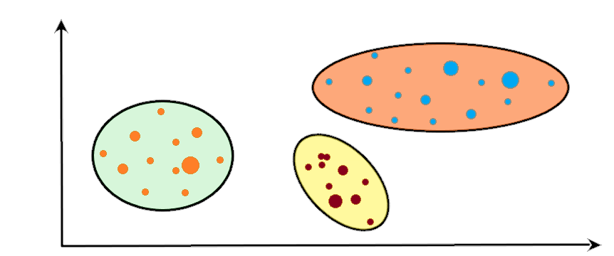
Since, clustering is the process of separating all data into groups (also known as collections) based on patterns in the data. We have no predictive target. We look at the details and try to make common sense and create different groups. It is therefore a problem of unsupervised learning.
SLIDING WINDOW METHOD:
In the sliding window method, a window of specified length, Len, moves over the data, sample by sample, and the statistic is computed over the data in the window. One cannot directly store the user image due to privacy policies, sketch of images are used. We simplify and improve the state-of-the-art of k-clustering sliding window algorithms, resulting in lower memory algorithms.

In the sliding window method, a window of specified length, Len, moves over the data, sample by sample, and the statistic is computed over the data in the window. One cannot directly store the user image due to privacy policies, sketch of images are used. We simplify and improve the state-of-the-art of k-clustering sliding window algorithms, resulting in lower memory algorithms.
The technique can be best understood with the window pane in bus, consider a window of length n and the pane which is fixed in it of length k. Consider, initially the pane is at extreme left i.e., at 0 units from the left. Now, co-relate the window with array arr[] of size n and pane with current_sum of size k elements. Now, if we apply force on the window such that it moves a unit distance ahead. The pane will cover next k consecutive elements.
Consider an array arr[] = {5, 2, -1, 0, 3} and value of k = 3 and n = 5
Applying sliding window technique:
We compute the sum of first k elements out of n terms using a linear loop and store the sum in variable window_sum.
Then we will graze linearly over the array till it reaches the end and simultaneously keeps track of the maximum sum.
To get the current sum of a block of k elements just subtract the first element from the previous block and add the last element of the current block.
The below representation will make it clear how the window slides over the array. This is the initial phase where we have calculated the initial window sum starting from index 0. At this stage, the window sum is 6. Now, we set the maximum_sum as current_window i.e 6.
Now, we slide our window by a unit index. Therefore, now it discards 5 from the window and adds 0 to the window. Hence, we will get our new window sum by subtracting 5 and then adding 0 to it. So, our window sum now becomes 1. Now, we will compare this window sum with the maximum_sum. As it is smaller we won't change the maximum_sum.
Similarly, now once again we slide our window by a unit index and obtain the new window sum to be 2. Again we check if this current window sum is greater than the maximum_sum till now. Once, again it is smaller so we don’t change the maximum_sum. Therefore, for the above array, our maximum_sum is 6. Now, it is quite obvious that the Time Complexity is linear as we can see that only one loop runs in our code. Hence, our Time Complexity is O(n).
Code:
# O(n) solution for finding
# maximum sum of a subarray of size k
def maxSum(arr, k):
# length of the array
     n = len(arr)
# n must be greater than k
 if n < k:
 print("Invalid")
 return -1
# Compute sum of first window of size k
     window_sum = sum(arr[:k])
# first sum available
     max_sum = window_sum
# Compute the sums of remaining windows by
# removing first element of previous
# window and adding last element of
# the current window.
 for i in range(n - k):
          window_sum = window_sum - arr[i] + arr[i + k]
          max_sum = max(window_sum, max_sum)
 return max_sum
# Driver code
arr = [1, 4, 2, 10, 2, 3, 1, 0, 20]
k = 4
print(maxSum(arr, k))
Code explanation:
Step 1: Let be a window of length n and the pane which is fixed in it of length be k. Consider, initially the pane is at extreme left i.e., at 0 units from left, and co-relate the window with array (arr[]) of size n and pane with current_sum of size k elements. Step 2: Consider an array arr[] = {5, 2, -1, 0, 3} and value of k = 3 and n = 5 Step 3: For applying the sliding window technique, first we compute the sum of k elements out of n terms using a linear loop and store the sum in variable window_sum. Step 4: Then we will graze linearly over the array till it reaches the end and simultaneously we will keep track of the highest sum. Step 5: For obtaining the current sum block of k elements, subtract the first element from the previous block and add the last element of the current block.
How to get the window sliding over the array?
Step 1: In the initial phase, we have calculated the initial window sum starting from index 0. At this stage, the window sum is 6. Now, we set the maximum_sum as current_window i.e 6. Step 2: Now it discards 5 from the window and adds 0 to the window. Hence, we will get our new window sum by subtracting 5 and then adding 0 to it. So, our window sum now becomes 1. Step 3: As we compared this window sum with the maximum_sum, it is smaller therefore we won’t change the maximum_sum. Step 4: Similarly, we once again slide our window by a unit index and obtain the new window sum to be 2. It will give us the same result as in Step 3 therefore we don’t have to change the maximum_sum Step 5: Therefore, for the above array our maximum_sum is 6. So it is quite obvious that the Time Complexity is linear as we can see that only one loop runs in our code. Hence, our Time Complexity is O(n).
K-MEANS CLUSTERING:
K-means algorithm identifies k number of centroids, and then allocates every data point to the nearest cluster, while keeping the centroids as small as possible.

Clustering points in a sliding window of a stream is a straightforward application of the clustering algorithm to each window. The algorithm uses the centroids of the clusters in each window as the initial estimates of the centroids in the following window. When the step size is small compared to the window size, the centroids of successive windows are likely to be close to each other. So, the algorithm converges more rapidly by starting with the previous window’s centroids rather than by starting with random points.
Code:
# k-means clustering
from numpy import unique
from numpy import where
from sklearn.datasets import make_classification
from sklearn.cluster import KMeans
from matplotlib import pyplot
def kmeans_sliding_windows(in_stream, out_stream, window_size, step_size, num_clusters):
   kmeans_object = KMeansForSlidingWindows(num_clusters)
   map_window(kmeans_object.func, in_stream, out_stream,window_size, step_size) # define dataset
X, _ = make_classification(n_samples=1000, n_features=2, n_informative=2, n_redundant=0, n_clusters_per_class=1, random_state=4)
# define the model
model = KMeans(n_clusters=2)
# fit the model
model.fit(X)
# assign a cluster to each example
yhat = model.predict(X)
# retrieve unique clusters
clusters = unique(yhat)
# create scatter plot for samples from each cluster
for cluster in clusters:
 # get row indexes for samples with this cluster
    row_ix = where(yhat == cluster)
# create scatter of these samples
pyplot.scatter(X[row_ix, 0], X[row_ix, 1])
# show the plot
pyplot.show()
Code Explanation:
Step 1: Here num_clusters is the number of clusters and kmeans_object is the object that keeps track on the centroids of the most recent window into the stream.
Step 2: kmeans_object.func is the function that computes the clusters of the next window by starting with the centroids of the previous window.
Step 3: As above example fits the model on the training dataset and predicts a cluster for each example in the dataset while running.
Step 4: Then a scatter plot is created with points colored by their assigned cluster.
Step 5: In this case, a reasonable grouping is found, although the unequal- equal variance in each dimension makes the method less suited to this data set.

Output Graph: 1000 point into 2 clusters
AUGMENTED MAYERSON SKETCH:
Step 1: Construct a set C of size O(k log Δ), (known as a sketch)
Step 2: Construct weighted instance such that, with constant probability
fp(X, C) ∈ O(OPTp(X))
Step 3: the success probability to be arbitrarily close to 1
Step 4: the latter’s weight is incremented by 1, when the new point does not make it as a centre
Step 5: The augmented Meyerson algorithm computes an implicit mapping μ : X → C, and a -consistent weighted instance (C,weight \) for all substreams X*τ,t+ with τ ≥ t−w, such that,with probability 1−γ
Step 6: we have: |C| ≤ 2 2p+8k log γ −1 log Δ and fp(X*τ,t+ , C) ≤ 2 2p+8 OPTp(X)
Step 7: Thus the algorithm uses space O(k log γ −1 log Δ log(M/m)(log M +log w+log Δ)) and stores the cost of the consistent mapping, f(X, μ), and allows a 1 + approximation which is denoted by fb(X*τ,t+ , μ).

Step 1: Start with treating each data point as one cluster, let number of clusters at the start be K, while K is an integer representing the number of data points.
Step 2: Form a cluster by joining the two closest data points resulting in K-1 clusters, same goes with more clusters resulting in K-2 clusters.
Step 3: Repeat the above two steps until one big cluster is formed.
Step 4: Once single cluster is formed, dendrograms are used to divide into multiple clusters depending upon the problem.
Different ways to find distance between the clusters:
Measure the distance between the closes points of two clusters. Measure the distance between the farthest points of two clusters. Measure the distance between the centroids of two clusters. Measure the distance between all possible combination of points between the two clusters and take the mean.
Code with explanation :
Step 1: Suppose we have a collection of data points: age vs average monthly health expenditure in hundred represented by a numpy array as follows:
Import numpy as np
X=np.array([[5,3],[10,15],[15,12],[24,10],[30,30],[85,70],[71,80],[60,78],[70,55],[80,91],])
Step 2: Let's plot the above data points.This code draws the data points in the X numpy array and label data points from 1 to 10:
import matplotlib.pyplot as plt
labels = range(1, 11)
plt.figure(figsize=(10, 7))
plt.subplots_adjust(bottom=0.1)
plt.scatter(X[:,0],X[:,1], label='True Position')
for label, x, y in zip(labels, X[:, 0], X[:, 1]):
  plt.annotate( label,xy=(x, y), xytext=(-3, 3),textcoords='offset points',ha='right', va='bottom')
plt.show() 
Step 3: To draw the dendrograms for our data points. We will use the scipy library for that purpose. Execute the following script:
from scipy.cluster.hierarchy import dendrogram, linkage
from matplotlib import pyplot as plt
linked = linkage(X, 'single')
labelList = range(1, 11)
plt.figure(figsize=(10, 7))
dendrogram(linked,orientation='top',labels=labelList,distance_sort='descending', show_leaf_counts=True)
plt.show() 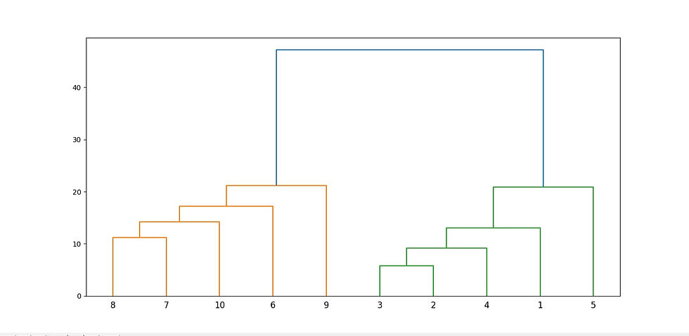
The output graph looks like the one above.
Step 4: The next step is to join the cluster formed by joining two points to the next nearest cluster or point which in turn results in another cluster. If you look at Graph1, point 4 is closest to cluster of point 2 and 3, therefore in Graph2 dendrogram is generated by joining point 4 with dendrogram of point 2 and 3. This process continues until all the points are joined together to form one big cluster.
Step 5: Once one big cluster is formed, the longest vertical distance without any horizontal line passing through it will be selected and a horizontal line is drawn through it.

Step 6: In above graph, we can see that the largest vertical distance without any horizontal line passing through it is represented by blue line. So we draw a new horizontal red line that passes through the blue line. Since it crosses the blue line at two points, therefore the number of clusters will be 2. Basically the horizontal line is a threshold, which defines the minimum distance required to be a separate cluster.

Step 7: In the above plot, the horizontal line passes through four vertical lines resulting in four clusters: cluster of points 6, 7, 8 and 10, cluster of points 3, 2, 4 and points 9 and 5 will be treated as single point clusters.
Introducing the first algorithms for the problem of k integration in sliding windows with line spaces in k. We strongly consider that the algorithm works much better than analytic parameters, and allows us to store only a small fraction of inputs. A natural way for future work is to provide a solid analysis, and to bridge this gap between theory and practice.
GitHub : https://github.com/rutujadoiphode913/sliding_window_algorithm_k_means_clustering
REFERENCES:
https://proceedings.neurips.cc/paper/2020/file/631e9c01c190fc1515b9fe3865ab bb15- Paper.pdf
https://en.wikipedia.org/wiki/Cluster_analysis
https://ieeexplore.ieee.org/stamp/stamp.jsp?arnumber=8501907
https://proceedings.neurips.cc//paper/2020/file/631e9c01c190fc1515b9fe3865a bbb15- Paper.pdf
Comments