Author - Simreeta Saha
The paper is based on SVM (Support Vector Machines). They are tools in Machine Learning. They are sets of supervised learning techniques used in classification, regression and outliers detection. It is used for creating the optimal decision boundary. We will further discuss about it in the later paragraphs.
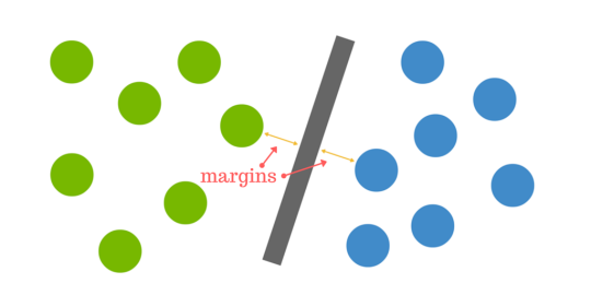
Figure_1
Support Vector Machine is an implementation of supervised learning technique which uses classification and regression algorithms for getting two groups. There are training data, {(x1, y1) ... (xn, yn)} in Rn x R which is sampled according to a unknown probability distribution P(x, y) and a generic loss function V(y, f(x)) that calculates the error, for a given x. f(x) is predicted in place of the actual value of y [3][4]

Figure: 1 The integration function [1]
This function minimizes the error. Next, we will see more about Support Vector Machine.
Support Vector Machine Model
Using SVM we generally modify a model from linear regression to a better prediction model by forming a curve-shaped graph. This is used for constructing hyper-planes in a multidimensional space [1] and the number of vectors used is called feature vectors of the dataset. We can use various feature selection techniques to get these feature vectors. So, we generally construct 3 lines:
w.x-b=0
w.x-b=1
w.x-b=-1
These together forms the hyperplane which can be optimized by maximizing the perpendicular distance between the lines.

Figure: 2 SVM Classifier [1]

Figure: 3 Non-Linear Classification
Hyper-Plane
In SVM approach, we make parallel partitions by parallel lines. This plane formed is called hyperplane. By maximizing the width between these two lines, we can optimize the Hyperplane. This is generally solved using Quadratic equation.[2]
SVMs can be called as probabilistic approaches but do not consider dependencies among the attributes. SVM works on empirical risk minimization which leads us to an optimization function as in:
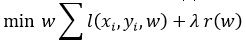
Where
l is the loss function (Hinge loss in SVMs) and
r is the regularization function.
SVM is a squared l2-regularized linear model i.e., r(w)= ∥ w2 ∥2.
Over-fitting
When number of features is much greater than the number of training data samples (m>>n), the regularization function introduces a bias so large that the training data model heavily under-performs causing over fitting.[1] [3] . It is therefore, mostly caused by dimensionality. This can be removed by proper selection of Kernel and proper tuning during regression.

Figure 4:
1st shows Linear Regression,
2nd shows almost perfect fit,
3rd show over-fit
Algorithm
There are two cases:
Separable
Non-Separable
But, the optimal solution is which gives the largest distance to the nearest observation given by the equation:
wx+b=0
This equation must satisfy the two conditions, one being it should separate the two classes A and B very well i.e., f (x) = ω. x + b is positive if and only if x ∈ A. And the other, it should exist further away from all the possible observations adding to the robustness of the model. Given that the distance from the hyper-plane to the observation x is
|ω.x+b|/||a||.
The maximum margin should be 2/||a||. Whereas in non-separable case the two classes cannot be separated properly, they overlap.[1]
Types of SVM Classifier
Linear SVM
Linear SVM actually means SVM with Linear Kernel. Here n datasets (x1, y1 to xn, yn) are used for training. A large margin classifier between the two classes of data is obtained. Any hyper-plane can be mentioned as the set of points 𝑥⃗ satisfying :


Figure 5: The equations for linear kernel
Non-Linear SVM
1. Polynomial Kernel function
It works on SVM that represents the similarity of the training samples in a feature space over polynomials of the original variables.[1] For degree d polynomials, the kernel works with the function in:
K(x,y) - (xy + C)
x, y are vectors in input space
C parameter to reduce the gap between higher orders and lower orders, if C=0, the function is homogeneous.
K is the inner product of the feature space based on a mapping φ i.e.
K(x,y) = < (φ (x) , φ (y)) >.

Figure 6: Response of the kernel function on different degrees(d=0, d=2, d=5)
2. Sigmoid Kernel function
Sigmoid Kernel Function can be trained to work for Gaussian RBF Kernels. In sigmoid kernel the performance of the kernel depends on the cross validation one needs to do. It finds it application as an activation function of artificial neurons as in equation:

Figure 7: Sigmoid function
3. Radial basis Kernel function
RBF is real valued function. It depends on Euclidean distance form origin:
Φ(x, c) = Φ(||x − c||)
It is used to calculate Euclidean distance between two coordinates based on the parameter σ:
K(x, x′) = exp (− γ||x − x′||2)
where,
γ =1 / 2σ2
So, γ is inversely proportional to σ.

Figure 8: Radial Basis function
Real Life application
1. Spam Filtering
2. Facial detection
3. Text Categorization
4. Bioinformatics
5. Predictive control of Environmental disasters
Git-hub Link :
Reference
A Study on Support Vector Machine based Linear and Non-Linear Pattern Classification by Sourish Ghosh, Anasuya Dasgupta, Aleena Swetapadma.
H. Han, J. Xiaoqian, “Overcome Support Vector Machine Diagnosis Overfitting.” Cancer Informatics, vol. 13, suppl 1, pp. 145–158, 2014.
J. Vert, K. Tsuda, and B. Schölkopf, "A primer on kernel methods", 2004.
https://datascience.foundation/sciencewhitepaper/underfitting-and-overfitting-in-machine-learning
Comments